Project 5 / Face Detection with a Sliding Window
For this project we implement a Face Detection algorithm using the popularly cited Dalal and Triggs 2005 detection pipeline. The procedure to object detection, specifically the special case face detection we implement here involves using a sliding window to scan the test image for matches with a pretrained HoG Histogram of Gradients classifer. To pre-train our HoG classifer we sample HoG features from training positive images containing faces as well as a set of negative features from randomly sampled negative images. We then comebine the positive and negative features into a single dataset and train our classifier with VL_SVMTRAIN() given a regularization parameter lambda and associated binary labels.
- Create positive and negative features from training images
- Train a linear classifier
- Mine Hard Negatives
- Create a multi-scale, sliding window face detector
Step 0. Baseline detection results
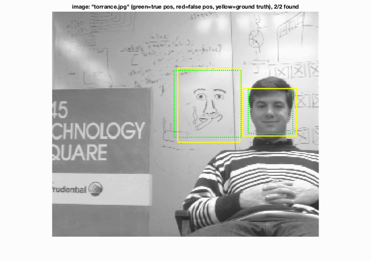
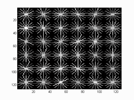
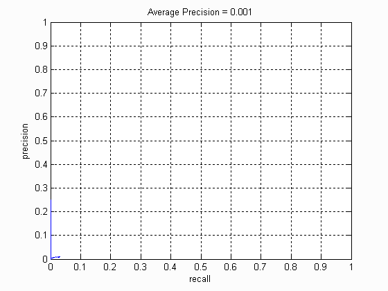
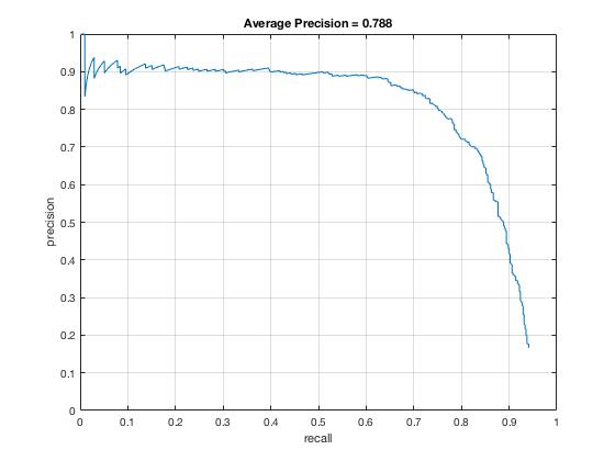
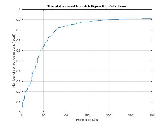
Without implementing anything at all, we get the following Face template HoG visualization for the starter code. This is completely random, but it should actually look like a face once you train a reasonable classifier. The graph on the right shows the Average Precision-Recall curve for the starter code.
Step 1. Using training images to create positive and and negative training HoG features
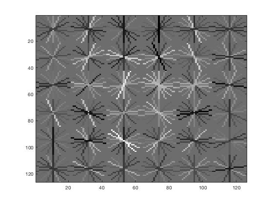
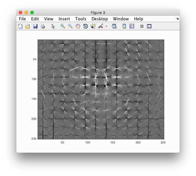
In the first stage of my face detection pipeline, I extract all Histogram of Gradients (HOG) of positive training images from the Caltech 101 Face imageset. I initially went with the defauly 36x36 pixel template size and 6x6 HoG cell size for balance between precision and computational efficiency. Once the positive features are extracted I proceeded to randomly sample negative features up to a budget threshold of 10000. Below is the Face template HoG visualization I get from just training on positive features of photos containing faces and combined with negative features of photos that don't have faces. We can observe that a pattern of gradients is starting to form.

Step 2. Train Linear SVM Classifier
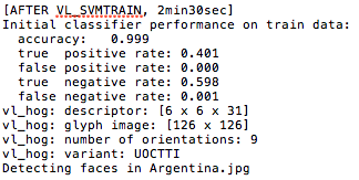
In step 2 of the procedure, we proceed to train a linear Support Vector Machine with a call to VL_SVMTRAIN. We choose a linear classifier here because its easy to implement yet relatively fast while yielding promising precision of detection. As we can see from our debugging statistics, the SVM fits very well to our training data with high accuracy.
lambda = 0.0001;
dataset =[features_pos; features_neg]';
labels =[ones(1, size(features_pos,1)), -ones(1, size(features_neg,1))];
[w, b] = vl_svmtrain(dataset, labels, lambda);
Step 3. Create a multi-scale, sliding window object detector.
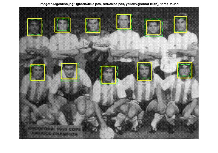
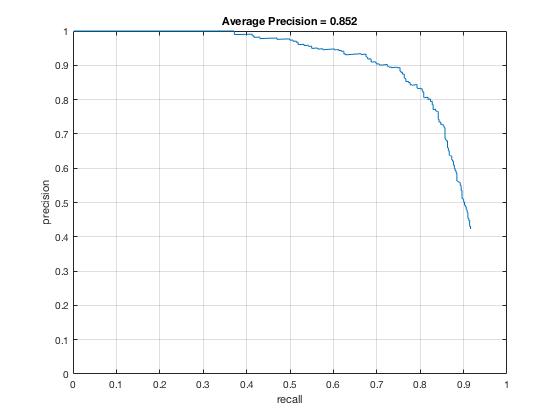
Once I had a linear SVM classifier working, I proceeded to designing the central algorithm of creating a sliding window, multi-scale detector. The following are my detection visualizations along with a much improved average precision curve, bringing it up from 78.8% to 85.2% vs. just using the linear SVM:
 ->
->
After experimenting with a variety of HoG cell sizes, I've come to the conclusion that a stepping size of 3 offers the best balance between average prediction precision and computational runtime. Below is the Face template HoG visualization with HoG cell size = 3 vs. 6.
Step 4. Extra Credits
- Implemented Hard Negative Mining
- Flipped HoG cells to use mirrors of input images expressed in HoG feature space as alternative positive training data
- Implemented a cascade architecture as in Viola-Jones, narrowing HoG cell size and detection threshold at every chained layer
- Test on Bonus data
Hard Negative Mining
I've implemented hard negative mining widely used in literature to show its effect on detection performance. The following three-point algorithm is used and we get the below visualization results.
% 1. Filter underqualified features from non-face images with SVM scores < -0.1
% 2. Compute hard negatives and augment the set of negative features found in step 1.
% 3. Retrain the linear SVM with this new augmented hard negatives.
if (hneg_on)
hneg_threshold = 10000;
[hneg_bboxes, hneg_conf, hneg_ids] = hneg_detector(non_face_scn_path, w, b, feature_params, hneg_threshold);
augmented_hneg = features_neg;

for i=1:size(hneg_conf,1)
    img = imread( fullfile( non_face_scn_path, char(hneg_ids(i)) ));
    img = im2single(img);
    if (size(img,3) > 1)
        img=rgb2gray(img);
    end

     % 'bboxes' is Nx4. N is the number of detections. bboxes(i,:) is
     % [x_min, y_min, x_max, y_max] for detection i.
     xmin = hneg_bboxes(i,1); xmax = hneg_bboxes(i,3);
     ymin = hneg_bboxes(i,2); ymax = hneg_bboxes(i,4);
     img=imcrop(img,[xmin,ymin,feature_params.template_size-1,feature_params.template_size-1]);

    % compute HoG feature
    hog = vl_hog(im2single(img), feature_params.hog_cell_size);
    k = size(hog(:)', 2); % debug info
    % augment negatives
    if (k == 1116)
        augmented_hneg = [augmented_hneg; hog(:)'];
    end
end

% retrain SVM
lambda = 0.0001;
hneg_dataset = [features_pos; augmented_hneg]';
hneg_labels =[ones(1, size(features_pos,1)), -ones(1, size(augmented_hneg,1))];
[w, b] = vl_svmtrain(hneg_dataset, hneg_labels, lambda);

end
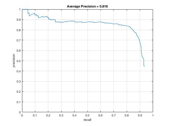
Notice how the Average Precision after implementing Hard Negatives have declined from 85.2% to 81.6%. Despite my effort to limit the amount of negative training data (having experimented with various budget of 5000, 7500 and 10000 negatives), the fact that the precision slipped agrees with the knowledge that because a linear classifiewr is not very exptessive, it doesn't necessary benefit from lots of hard negatives. Indeed, since our hard negatives in the training data are not particularly represenative of hard negatives in our test data coming from different databases (Caltech 101 vs. CMU+MIT), I've manually added in more non-face training scenes from the Caltech 101 database (sampled from different categories that are as far as possible from human faces, so I tried to stay away from animal faces) to improve the precision from < 80% to 81.6%.
(Selection of) Additional Negative Training Data


Alternative Positive Training Data
As another extra credit implementation, I've generated alternative training data by manipulating the original input data set in HoG feature space, i.e. usingVL_HOG()'s permutation variant parameter to flip HOG from left to right. Quoted from VL_FEAT's official website:
Often it is necessary to flip HOG features from left to right (for example in order to model an axis symmetric object). This can be obtained analytically from the feature itself by permuting the histogram dimensions appropriately. The permutation is obtained as follows:
% Get permutation to flip a HOG cell from left to right
perm = vl_hog('permutation') ;

% Then these two examples produce identical results (provided that the image contains an exact number of cells:
imHog = vl_hog('render', hog) ;
imHogFromFlippedImage = vl_hog('render', hogFromFlippedImage) ;
imFlippedHog = vl_hog('render', flippedHog) ;
Surprisingly, by producing twice the amount of positive training images this way, which refines the symmetricity of the HoG features to the lineae SVM, I was able to see about a 6-7% improvement in detection precision performance:

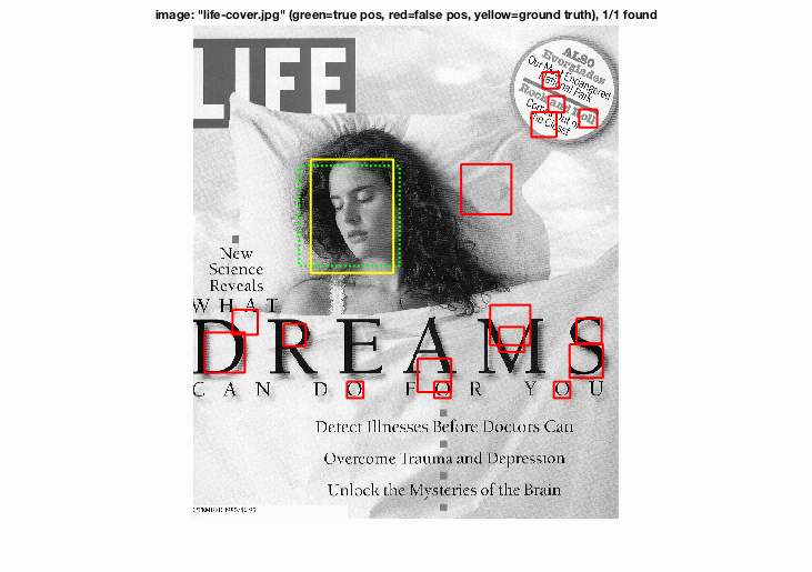
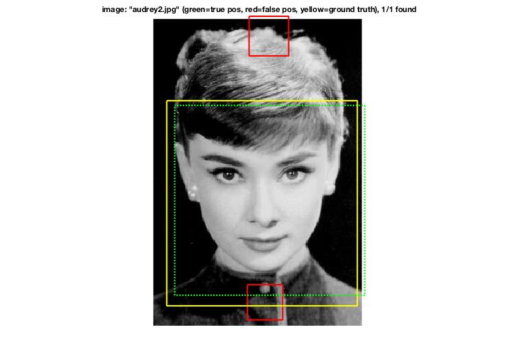
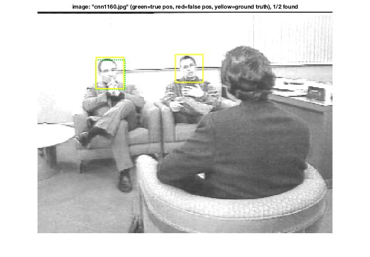
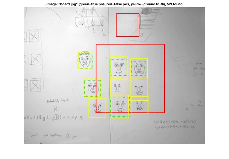
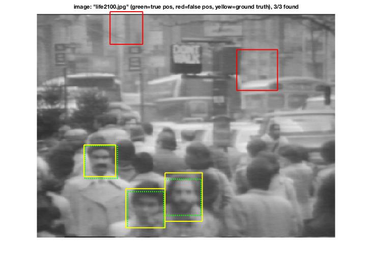
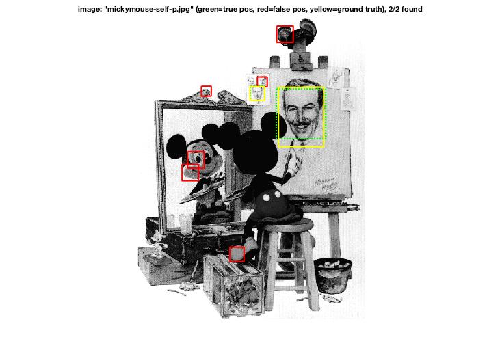
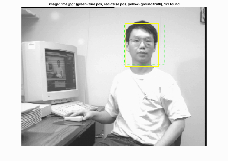
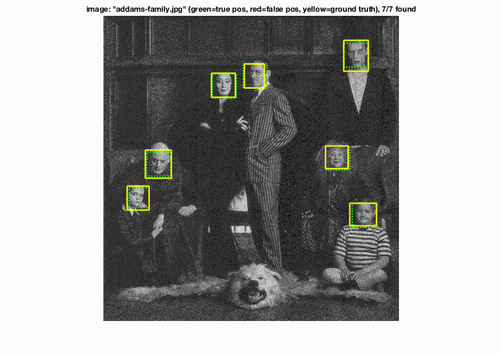
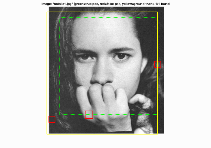
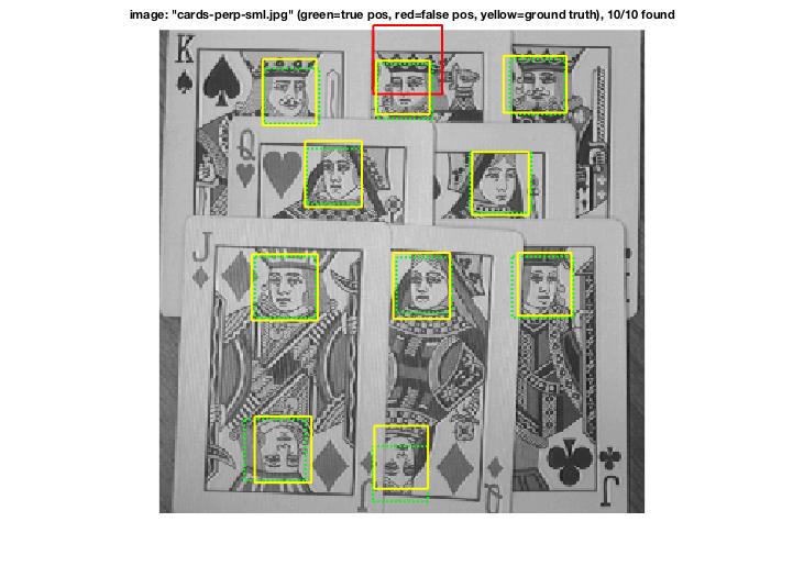
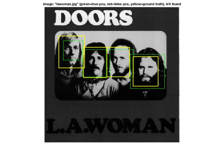
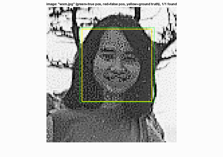
Combined with mining Hard Negatives, the following are some detection visualizations:
Cascade Architecture as in Viola-Jones.
In proj4_casecade.m and other *_cascade.m
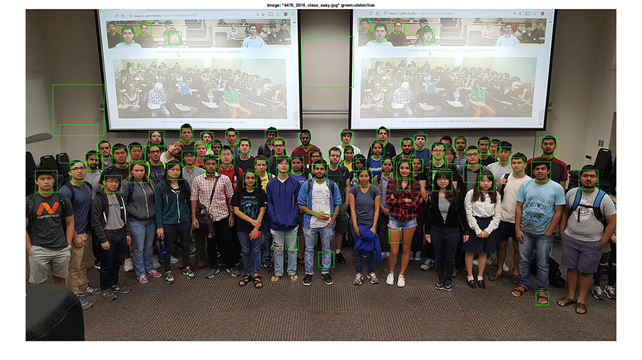
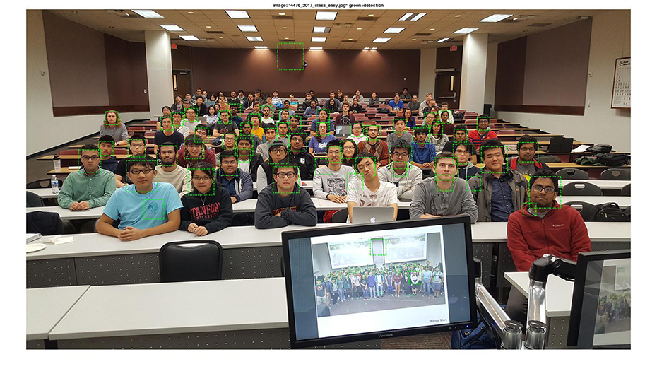
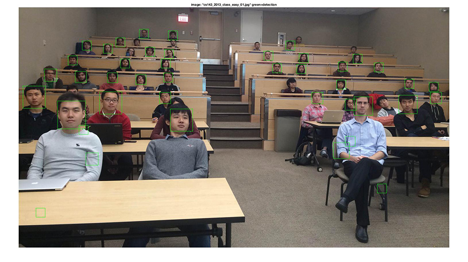
Some highlight results from 92.6% Average Precision
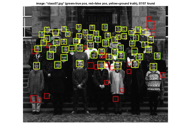
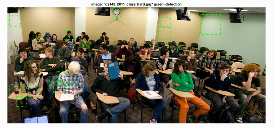
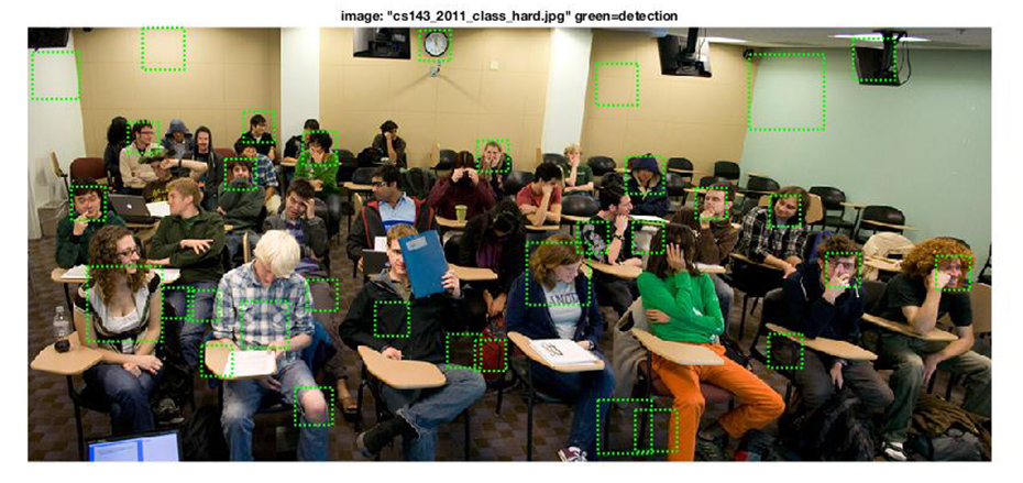
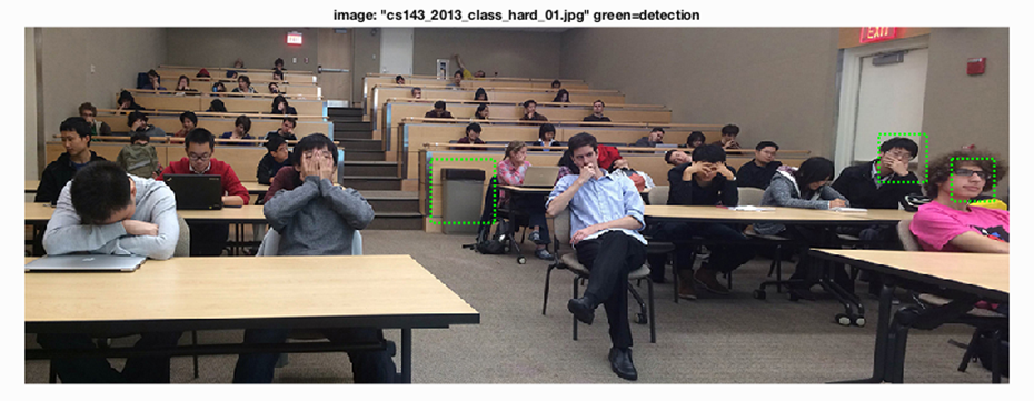
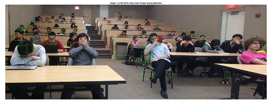
Bonus test scenes of Computer Vision class - confirmed Best-in-class
before vs. after (hard cases subject to occlusion)