Project 2: Local Feature Matching
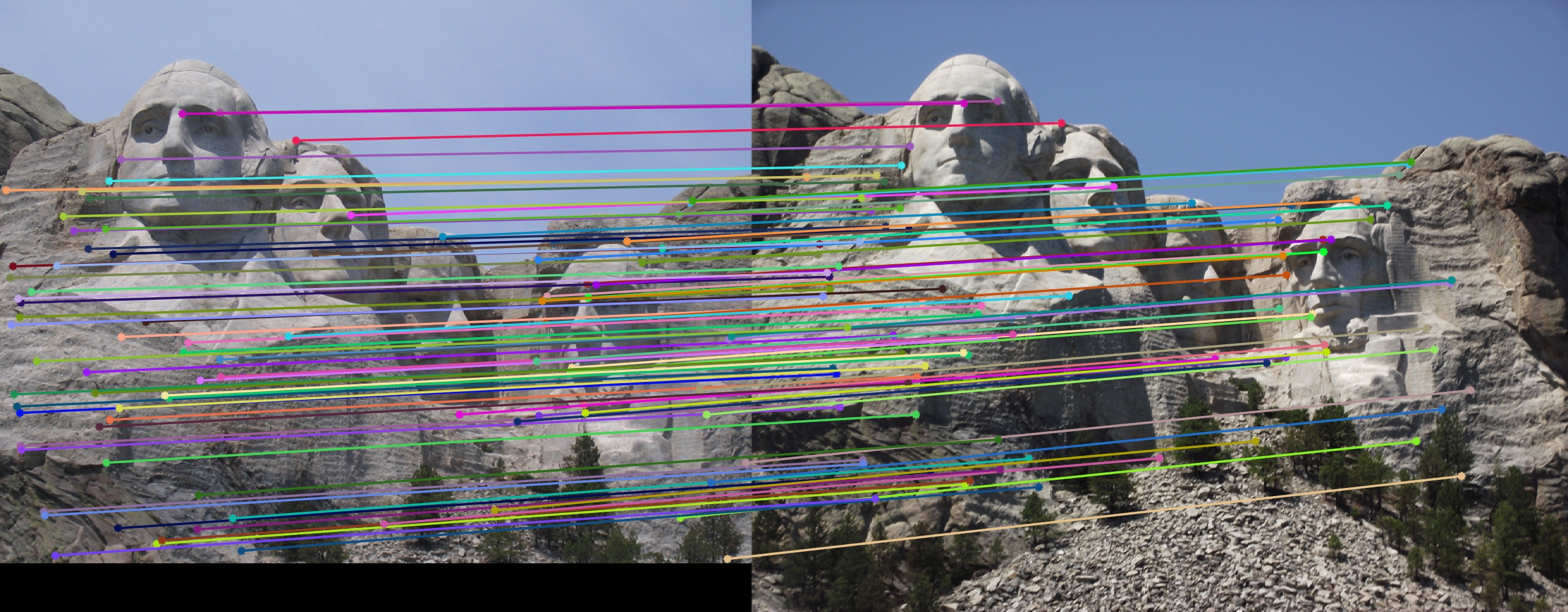
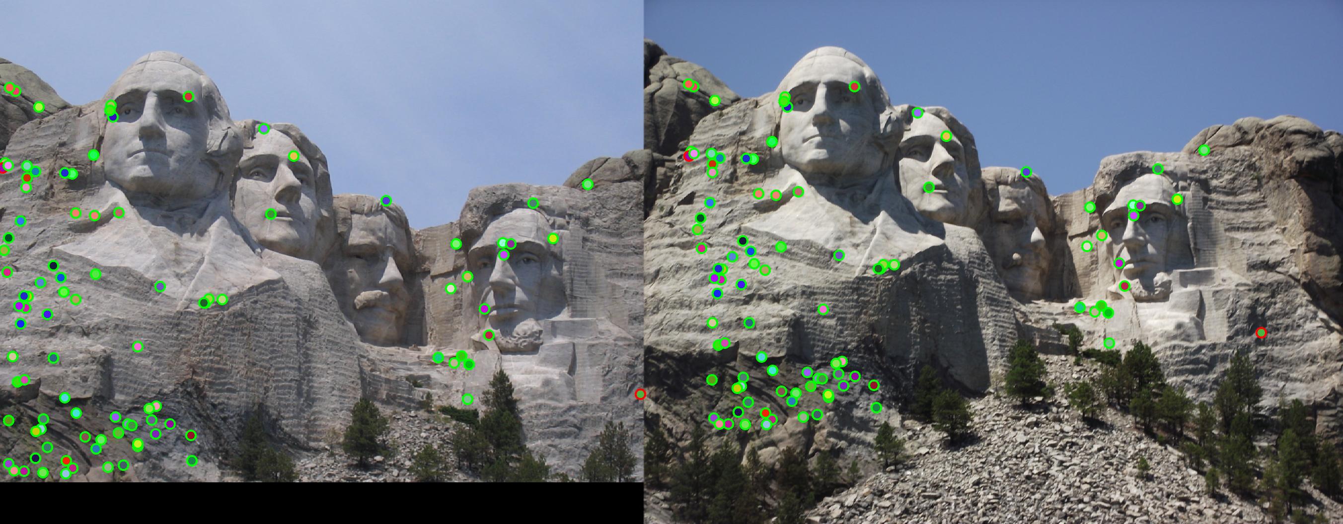
Fig 1. Feature matching for Mount Rushmore achieving 98% accuracy with KNN
In this project two images describing the same object are fed into a SIFT pipeline developed and visualized in MATLAB. Using the groundtruth evaluation code, I was able to gradually improve my image detection and matching algorithm both in its accuracy and efficiency. A couple main strategies include parameter tuning, expansion on textbook subprocedures (adaptive non-maximum suppression) and the introduction of alternative implementation strategies, all of which I will detail below.
Feature Detection w/ Harris Detector
For the initial stage of my SIFT pipeline I implemented the Harris corner detection algorithm to first localize points of interest (aka. "interest" points) in both images separately. Note that while this part differs from David Lowe's original SIFT detection algorithm, with some additional finetuning and alternative approximation we are able to still achieve robust results our testing images. The high-level implementation mainly follows from Georgia Tech's OMSCS CS6476 video lecture by Professor Aaron Bobick. The steps are conveniently shown below.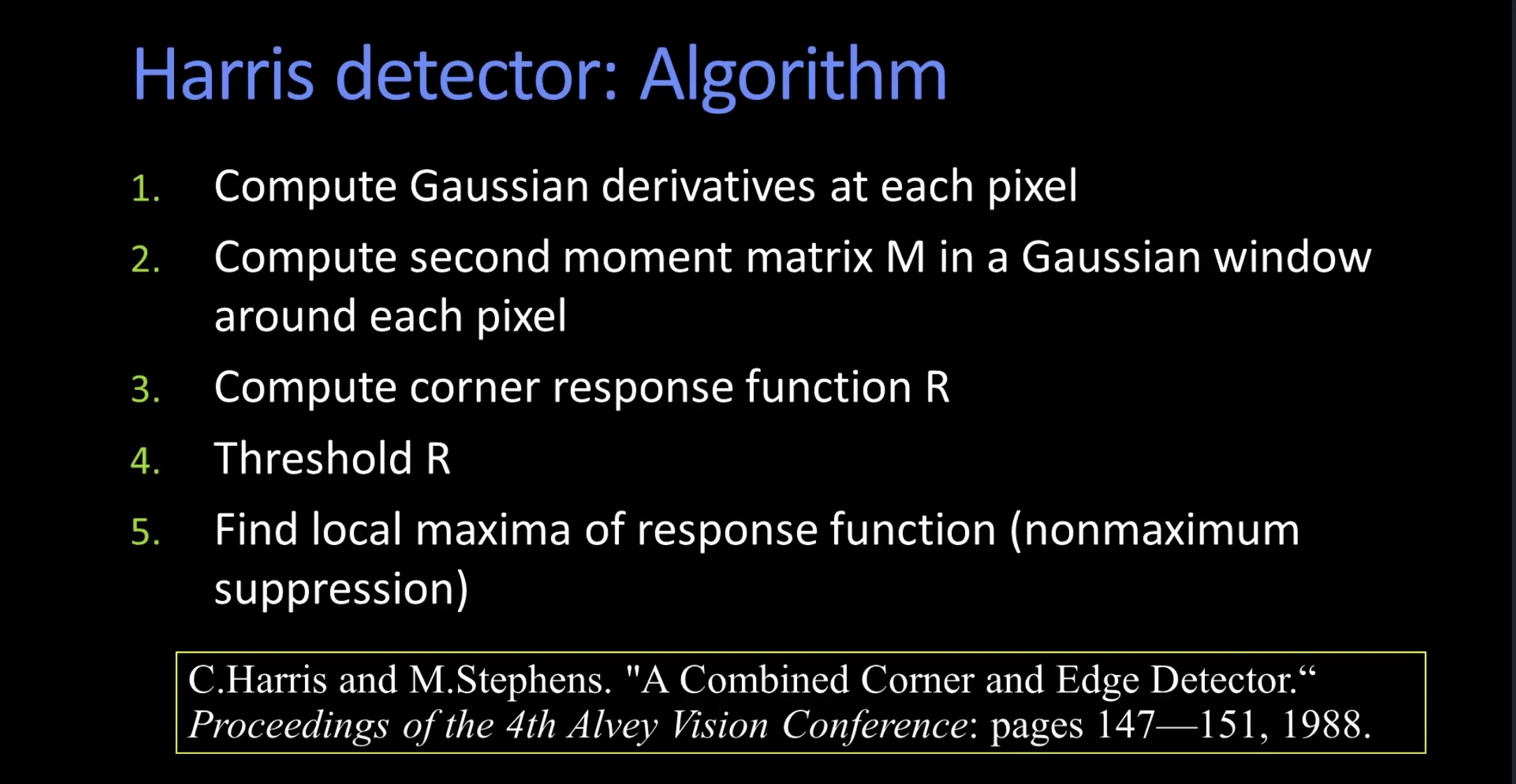
In
get_interest_points, my corner detection implementation computes the entries of second momement matrix M by taking the x- and y-gradients of the input image and multiplying them creatively followed by a gaussian convolution. The following snipper shows that we can using first-order derivatives to approximate values for second-order derivatives and subsequently the Harris corner response function in a very efficient manner.
% Harris Response Function R = det(M) - alpha*trace(M)^2 is approximated by
Response = (Ixx .* Iyy) - Ixy.^2 - a * (Ixx+Iyy).^2;
% where eigenvalus Ixx, Iyy = squaring input image's first-order derivatives Ix, Iy
% respectively and Ixy = Ix .* Iy. Alpha = 0.04 was found to be most effective.

% To neutralize overdetection of point clusters due to regions of high intensity
% we smooth the derivatives with a gaussian filter in which I fine-tuned its parameters
% window size and sigma radius to maximize detection accuracy
gaussD = fspecial('gaussian', [3 3], 2);
- My final implementation uses MATLAB's
bwconncomp()to iterate through every connected component to manually evaluate the maximum value of each connected component. - Experimentatation: I tried to include 2nd highest cornerness value of each connected component along with the max in my final interest points vector to see if it'll yield most interest points. By playing around, the observation made is that for most images this actually decreases matching accuracy as these secondary points tend to not be centered at corners and there're other parameters to yield more interest point detected (see commented code)
- Attempted Adaptive Non-maximum Suppression (ANMS) in addition to the normal non-maximum suppression which can be implemented with a MATLAB shortcut: simply calling
imregionalmaxon the response function will globally suppress non-maxima to 0s and bump maximal values to 1, producing a binary image of 0s and 1s. - Originally I hoped to accomplish ANMS by calling
COLFILT()with a given window size and the handy builtinimregionalmax()function. However due to underlying space inefficiencies ofimregionalmax()making unnecessary copies of the entire matrix MATLAB throws an exception dealing with ~16GB of matrices. I proceeded to manually implement ANMS with starting window radius = infinity decreasing to a small power of 2. (Powers of 2 is used to maximize computation efficiency) In every iteration the radius decreases by 1) linear steps of 32. 2) division factor of 2, 4. Yet through empirical testing I found this to be very time-consuming with a double for loop and because it took 30 seconds to 5 minutes for Notre Dame, I resorted to a fixed size window described in step 1.
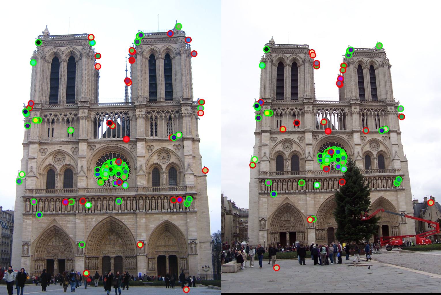
Fig 2. Feature detection for Notre Dame with non-maximum suppression. (notice ring near center)
Feature Description
A key stage of the SIFT pipeline is constructing the feature descriptor. My implementation follows the suggested algorithm found in Professor Hays's Lecture slides and the Szeliski textbook. The image had to be padded in all sides to accomodate for the sliding 16x16 window that computes a gradient histogram of 8 bins that describes the dominant gradient of all pixels within a 4x4 subcell. Everything is pretty straightforward and standard here except for fine-tuning the gaussian parameters and some improvements to optimize the descriptor's effectiveness.
Note:
- Gradient magnitudes are smoothed by a Gaussian fall-off function with sigmoid fine-tuned to roughly = 5
- I explicitly computed the gradient orientation at each pixel. The 16x16 window is split into 4 MATLAB cells and assigned component gradients by numerical scaling and division.
- Interestingly, using
ceil()instead ofround()when calculating each pixel's orientation contribution (each 45 degrees apart) improves final matching accuracy of Notre Dame from ~88% to 90+%. - Went with normalize -> threshold -> normalize to help descriptor effectiveness
- Normalized feature descriptor to unit vector, clipped descriptor entries at 0.2 and raised entry to power k < 1. Another parameter to play around! Found k = 0.6 to give highest accuracy.
Feature Matching
This part takes the feature descriptors from the last stage and finds matching between sets of descriptors of the two images by some method of distance evaluation. Calculating the nearest neighbor distance ratio (NNDR) from the textbook was rather straightforward, so I went with the following extensions:
Extra credit:
- Using MATLAB's K-Nearest Neighbor (KNN) alogirthm
knnsearch()to achieve optimal performance. Also trieddsearchn(), but it only gives x coordinates back and not corresponding y so I had to pivot. - Experimented with NNDR with not just the second closest matching feature but a combination of 1st-3rd, 2nd-3rd, and so forth. The conclusion was that for some images and combination of parameters in feature detection that yielded generally low number but more accurate keypoints, it actually improved overall matching effectiveness as it yields lower number false negatives, but in most cases accuracy went down by a bit.
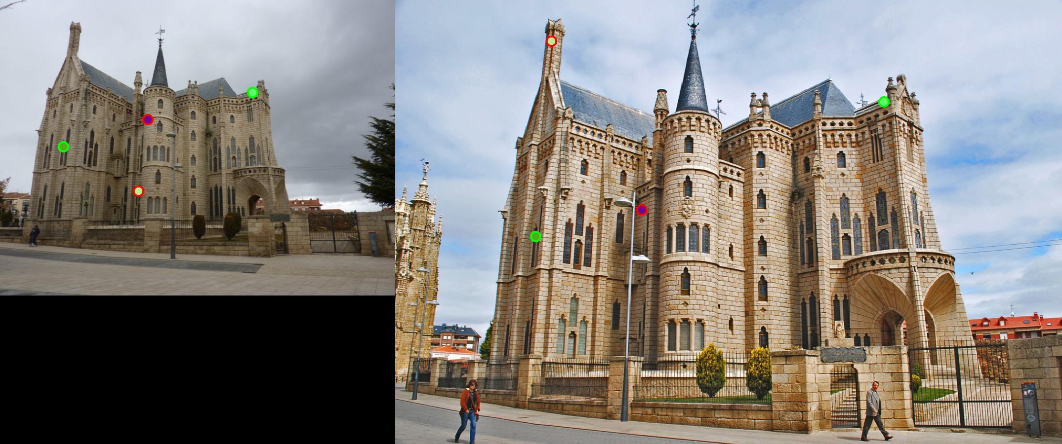
- Experimented with SIFT parameter Nearest Neighbor Distance Ratio threshold extensively in this matching stage and around that for Notre Dame, a threshold of = 0.9 was actually better with 96% accuracy (vs. 91%) whereas for the hardest image Episcopal Gaudi, changing threshold from 0.9 to 0.8 actually improved accuracy from 14% to 55%.
- Create a lower dimensional descriptor that is still accurate enough. By running Principle Component Analysis (PCA) on the original 128 feature vector and extracting the eigenvectors of the coefficient matrix, we can use the eigenvalues from PCA to compress our feature vector by factors of 2 to fasten the matchijng process. In
proj2.mI've included a dimension reduction factor variable that makes it very easy to see the differences.
Results in a table
| Image Pair | Accuracy (NNDR, threshold = 0.85) | Accuracy (KNN matching) |
|---|---|---|
|
91.60% | 66.00% |
|
96.54% | 98.00% |
|
50.00% | 7.00% |
Time comparison between NNDR vs. KNN matching:
| Image | NNDR | NNDR+PCA (dim=64) | NNDR+PCA (dim=32) | KNN | KNN+PCA (dim=64) | KNN+PCA (dim=32) |
|---|---|---|---|---|---|---|
| Notre Dame | 16.62 secs | 18.50 secs | 19.85 secs | 10.33 secs | 9.93 secs | 9.69 secs |
| Mount Rushmore | 1 min 05.35 secs | 1 min 03.15 secs | 1 min 00.83 secs | 29.45 secs | 28.79 secs | 29.80 secs |
| Episcopal Gaudi | 21.43 secs | 19.43 secs | 19.98 secs | 14.90 secs | 13.58 secs | 13.70 secs |
Accuracy comparison between NNDR vs. KNN matching:
| Image | NNDR | NNDR+PCA (dim=64) | NNDR+PCA (dim=32) | KNN | KNN+PCA (dim=64) | KNN+PCA (dim=32) |
|---|---|---|---|---|---|---|
| Notre Dame | 91.60% | 88.12% | 59.38% | 66.00% | 75.00% | 62.00% |
| Mount Rushmore | 96.54% | 83.82% | 72.60% | 98.00% | 98.00% | 95.00% |
| Episcopal Gaudi | 50.00% | 20.00% | 5.66% | 7.00% | 6.00% | 7.00% |
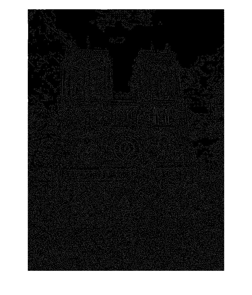
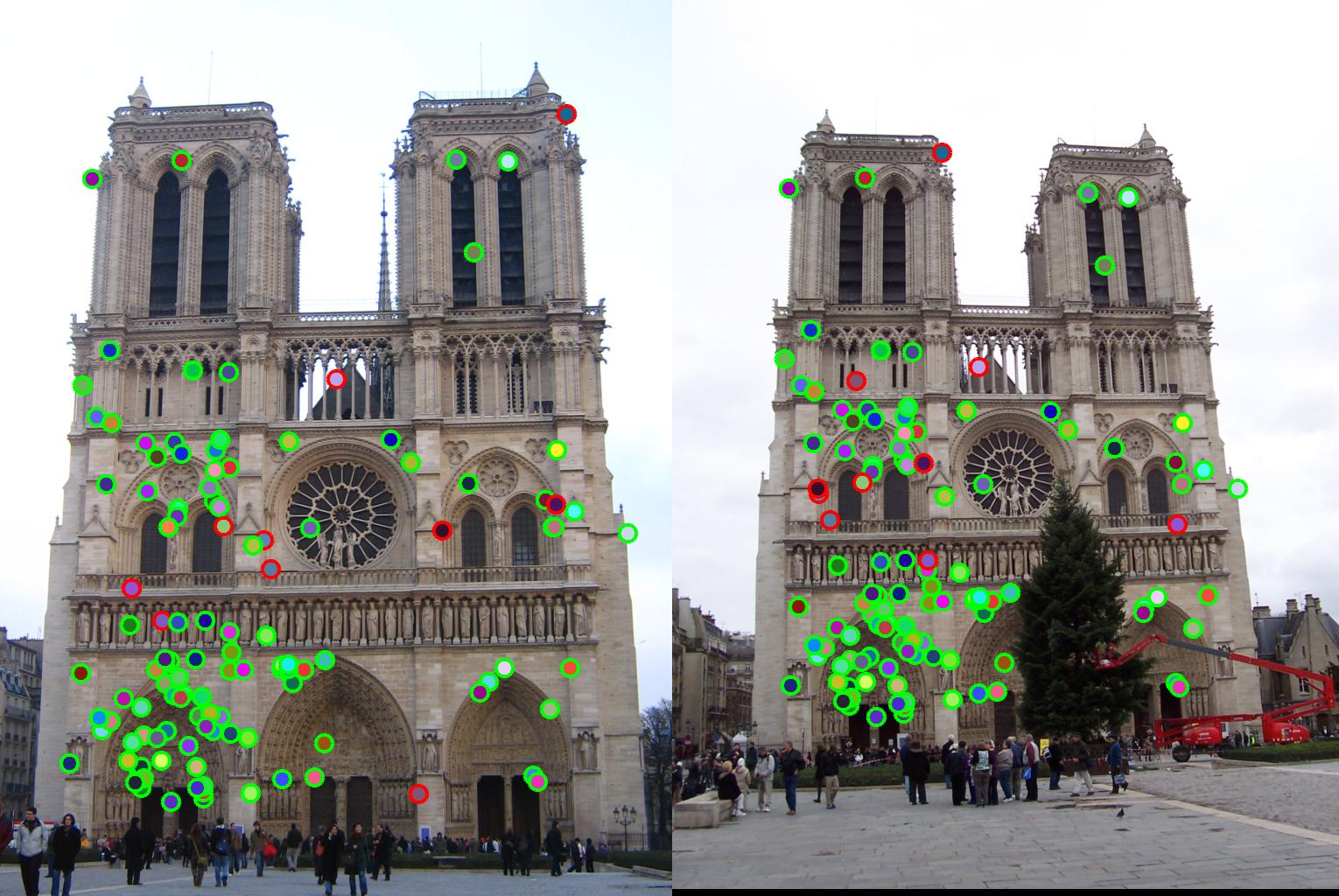
Fig 3. (Intermediate Binary) Thresholded Cornerness Detection for Notre Dame
Interesting Findings
- It's particularly amusing to notice some unexpected results. For instance, perhaps because PCA is only applied at the feature matching stage, we don't see a time improvement and in most cases actually observe a worsened time (due to the extra step of dimensionality reduction maybe?) across the board.
-While using the KNN matching strategy excelled at Mount Rushmore, it dropped matching accuracy rates for the other images quite significantly.
- Using KNN definitely yield noticeable if not significant time savings for all images, though as in the case of NNDR matching, applying PCA in our case did not help much.